Evaluating and using the adjustment weights
After weights are fitted in order to balance the sample, the results should be evaluated so to understand the quality of the weighting.
Summary statistics
Summary
Printing the adjusted object gives a high level overview of the content of the object:
print(adjusted)
Output:
        Adjusted balance Sample object with target set using ipw
        1000 observations x 3 variables: gender,age_group,income
        id_column: id, weight_column: weight,
        outcome_columns: happiness

        adjustment details:
            method: ipw
            weight trimming mean ratio: 20
            design effect (Deff): 1.880
            effective sample size proportion (ESSP): 0.532
            effective sample size (ESS): 531.9

            target:

            balance Sample object
            10000 observations x 3 variables: gender,age_group,income
            id_column: id, weight_column: weight,
            outcome_columns: happiness

            3 common variables: gender,age_group,income
To generate a summary of the data, use the summary method:
print(adjusted.summary())
This will return several results:
- Adjustment details: method used and weight trimming parameters
- Covariate diagnostics: ASMD is "Absolute Standardized Mean Difference". For continuous variables, this measure is the same as taking the absolute value of Cohen's d statistic (also related to SSMD), when using the (weighted) standard deviation of the target population. For categorical variables it uses one-hot encoding. Also includes KLD (Kullback-Leibler divergence) metrics.
- Weight diagnostics: Design effect, effective sample size proportion (ESSP), and effective sample size (ESS)
- Outcome weighted means: means for each outcome variable across self (adjusted), target, and unadjusted samples
- Model performance: Model proportion deviance explained (if inverse propensity weighting method was used)
Output:
Adjustment details:
    method: ipw
    weight trimming mean ratio: 20
Covariate diagnostics:
    Covar ASMD reduction: 63.4%
    Covar ASMD (7 variables): 0.327 -> 0.120
    Covar mean KLD reduction: 95.3%
    Covar mean KLD (3 variables): 0.071 -> 0.003
Weight diagnostics:
    design effect (Deff): 1.880
    effective sample size proportion (ESSP): 0.532
    effective sample size (ESS): 531.9
Outcome weighted means:
            happiness
source
self           53.295
target         56.278
unadjusted     48.559
Model performance: Model proportion deviance explained: 0.173
Note that although we had 3 variables in our original data (age_group, gender, income), the asmd counts each level of the categorical variables as separate variable, and thus it considered 7 variables for the covar ASMD improvement.
Covariate Balance
We can check the mean of each variable before and after applying the weights using .mean():
adjusted.covars().mean().T
To get:
source self target unadjusted
_is_na_gender[T.True] 0.086776 0.089800 0.088000
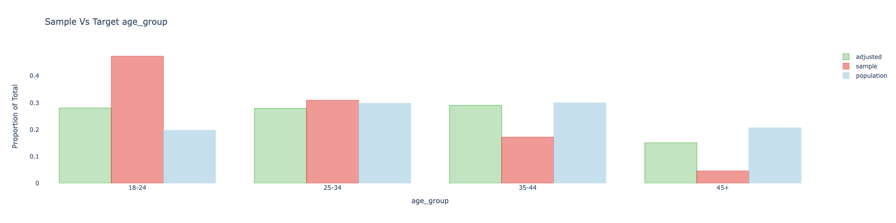
age_group[T.25-34] 0.307355 0.297400 0.300000
age_group[T.35-44] 0.273609 0.299200 0.156000
age_group[T.45+] 0.137581 0.206300 0.053000
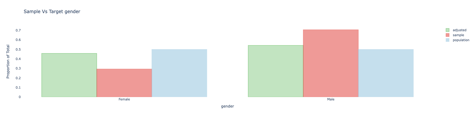
gender[Female] 0.406337 0.455100 0.268000
gender[Male] 0.506887 0.455100 0.644000
gender[_NA] 0.086776 0.089800 0.088000
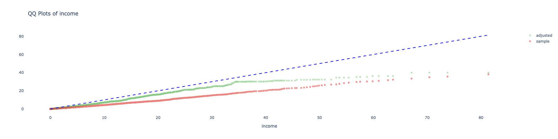
income 10.060068 12.737608 6.297302
Here, self is the adjusted (weighted) covariate mean, target is the target mean, and unadjusted is the unadjusted sample mean.
And .asmd() to get ASMD:
adjusted.covars().asmd().T
To get:
source                  self  unadjusted  unadjusted - self
age_group[T.25-34]  0.021777    0.005688          -0.016090
age_group[T.35-44]  0.055884    0.312711           0.256827
age_group[T.45+]    0.169816    0.378828           0.209013
gender[Female]      0.097916    0.375699           0.277783
gender[Male]        0.103989    0.379314           0.275324
gender[_NA]         0.010578    0.006296          -0.004282
income              0.205469    0.494217           0.288748
mean(asmd)          0.119597    0.326799           0.207202
We can see that on average the ASMD improved from 0.33 to 0.12 thanks to the weights. We got improvements in income, gender, and age_group.
Although we can see that age_group[T.25-34] and gender[_NA] didn't improve.
Understanding the model
For a summary of the diagnostics measures, use:
adjusted.diagnostics()
This will give a long table that can be filterred to focus on various diagnostics metrics. For example, when the .adjust() method is run with model="ipw" (the default method), then the rows from the diagnostics output with metric == "model_coef" represent the coefficients of the variables in the model. These can be used to understand the model that was fitted (after transformations and regularization).
Visualization post adjustments
We can create all (interactive) plots using:
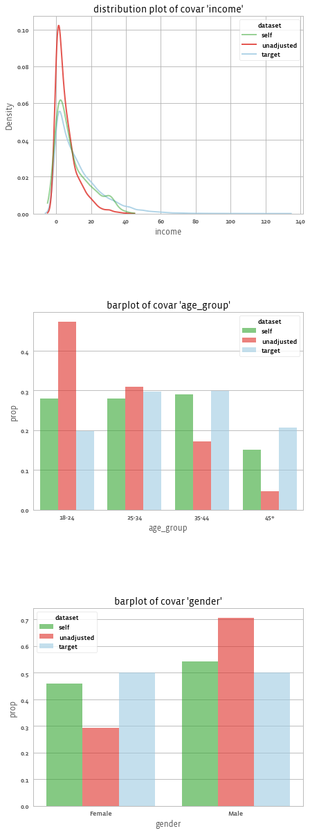
adjusted.covars().plot()
And get:
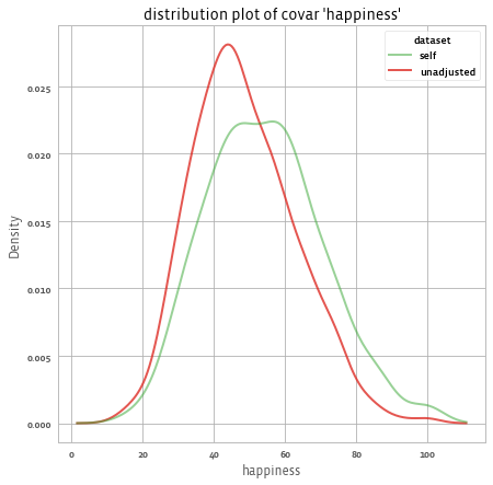
We can also use different plots, using the seaborn library, for example with the "kde" dist_type.
adjusted.covars().plot(library = "seaborn", dist_type = "kde")
And get:
Distribution of Weights
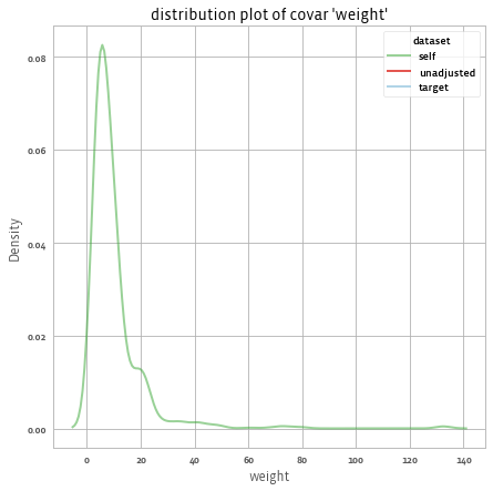
We can look at the distribution of weights using the following method call:
adjusted.weights().plot()
And get:
Or calculate the design effect using:
adjusted.weights().design_effect()
# 1.88
Analyzing the outcome
The .summary() method gives us the response rates (if we have missing values in the outcome), and the weighted means before and after applying the weights:
print(adjusted.outcomes().summary())
To get:
1 outcomes: ['happiness']
Mean outcomes (with 95% confidence intervals):
source       self  target  unadjusted           self_ci         target_ci     unadjusted_ci
happiness  53.295  56.278      48.559  (52.096, 54.495)  (55.961, 56.595)  (47.669, 49.449)
Note: The target column and target-based response rates appear only when the target Sample has outcome data. If your target has no outcomes, you will only see self and unadjusted columns.
Weights impact on outcomes (t_test):
           mean_yw0  mean_yw1  mean_diff  diff_ci_lower  diff_ci_upper  t_stat  p_value       n
outcome
happiness    48.559    53.295      4.736          1.312          8.161   2.714    0.007  1000.0

Response rates (relative to number of respondents in sample):
   happiness
n     1000.0
%      100.0
Response rates (relative to notnull rows in the target):
    happiness
n     1000.0
%       10.0
Response rates (in the target):
    happiness
n    10000.0
%      100.0
For example, we see that the estimated mean happiness according to our sample is 48.6 without any adjustment and 53.3 with adjustment (compared to the target mean of 56.3). The following shows the distribution of happiness before and after applying the weights:
adjusted.outcomes().plot()
Impact of weights on outcomes
To assess whether weighting statistically shifts the outcomes, compare the paired
products y*w0 versus y*w1. The helper below uses a paired t-test and reports
the baseline means, the mean difference, and its confidence interval:
adjusted.outcomes().weights_impact_on_outcome_ss(method="t_test")
You can also include this in the printable summary (enabled by default):
print(adjusted.outcomes().summary())
In diagnostics output, these appear under weights_impact_on_outcome_* metrics
by default (set weights_impact_method=None to disable in the summary, or
pass weights_impact_on_outcome_method=None when calling diagnostics).
To compare two adjusted models (for example, IPW vs. CBPS) on the same outcomes, use:
from balance.stats_and_plots.impact_of_weights_on_outcome import (
    compare_adjusted_weighted_outcome_ss,
)

compare_adjusted_weighted_outcome_ss(adjusted_ipw, adjusted_cbps)
And we get: